Resolving Eulerian path with inchrosil

Eulerian paths could define as graph which visits every edge exactly once, with singularity starts and ends on the same vertex. Therefore, an Eulerian path is a cycle which contains all edges of a graph just once. This problem was posed and resolved by Leonhard Euler himself in 1736 in a problem which has the name of the seven bridges of the city of Königsberg. The problem is enunciated in the following form: two islands in the Pregel River, in Königsberg are joined together and with land by seven bridges.

• Is it possible to take a walk starting by any of the four parts of land, crossing each one of the bridges just once?

Euler approached the problem representing each part of land by one point and each bridge by a line, joining the corresponding dots. Then, the previous problem can be transferred to the following question:

• Is it possible to travel round the representation without repeating the lines?

Euler demonstrated that it was not possible because the number of lines that affect each dot is uneven (a necessary condition to be able to enter and exit each dot). Therefore, this problem posed questions such as the following;

• How is it possible to cover the cable of this electricity grid without repeating sections of grid?
• How can this route be performed, passing through specific streets?

There is a complexity to solve these cycles’ problems, by this reason, we have considered inversely, i.e. all vertices could be converted in edges and all edges could be converted in vertices, with simple conversion, we can calculate any Hamiltonian path associated of conversion. On the other hand, since now the vertices represent the edges and it is necessary to know what sequence of vertices we should follow to be able to pass through all the edges.

Let us suppose the directed and non-weighted graph of Figure 1, which would be a multi-graph, i.e. a non-deterministic automaton.

Figure 1: Eulerian path.

The graph of Figure 8 can also be represented as follows, where V₁ is the set of vertices and E₁ is the set of edges.

G₁=(V₁,E₃) with V₁=(v₁,v₂,v₃) and E₁=(a₁,a₂,a₃,a₄,a₅,a₆)

Furthermore, we have the following vertex links, by means of edges;

U={(v₁,v₂,a₁),(v₁,v₂,a₂),(v₁,v₂,a₃),(v₂,v₃,a₄),(v₂,v₃,a₅),(v₂,v₃,a₆),(v₃,v₁,a₆)}

Where the nomenclature used for these links is (source vertex, destination vertex, edge). If said inversion is made, and if the edges are considered as vertices and the vertices as edges, we would obtain the following graph.

G₂=(V₂,E₂) with V₂=(a₁,a₂,a₃,a₄,a₅,a₆) and E₂=((v₁,v₂),(v₂,v₃),(v₃,v₁))

Furthermore, we have the following vertex links, by means of edges;

W= {(a₁, v1, v2, v2, v3, a4) . . .}

Therefore, the graph will have the form shown in Figure 1. Consequently, if the Hamiltonian path of the previous graph G₂ is shown, it can be stated that there is a solution or Eulerian path G₁. It can also be considered that the graph is weighted, the total costs of each one of the paths can be calculated and, therefore, sorted by cost, although the Eulerian paths do not have weight, new problems of optimization in the Eulerian paths could be posed. In conclusion, if a Hamiltonian path exists in graph G₂, it can be stated that there is an Eulerian path in graph G₁. Finally, it can be stated that Eulerian cycles can be resolved, for which purpose, when encoding the base of strands or banks of strands, it was established that the initial node was the same as the final. In this way, cycle problems can be resolved using the Hamiltonian Path device.

Resolving Travelling Salesman Problem with Inchrosil

The travelling salesman problem (TSP) is one of the most famous and best studied in the computational area, being one the most difficult to resolve, due its complexity, which is considered a NP-complete problem. In the previous section, we have described an electronic system to solve Hamiltonian path problem with a cost approximately of polynomial order, in this paragraph, the graph to analyze has a weighted and direction in its paths, where only one or set Hamiltonian paths are solution of TSP, so first step would be found all Hamiltonian paths at the graph, and next steps would be calculated final cost each Hamiltonian path found, using its weighted and directions, by this reason, in our research, we have used the same infrastructure explained in Hamiltonian Path device, which would obtain all Hamiltonian paths, later with these paths, the system would calculate each individual cost and compare all cost to get which is the best Hamiltonian path, always depending a initial characteristics established by programmer/user.

All these calculations could be done in parallel, also all criteria to sort path cost could be stored in different modules of the system, in this way any operation is quick and faster to do. In this article, we have considered two different systems to do all mathematical operation and choice the best Hamiltonian path cost, depending one specific criteria. The first system contains software to calculate and storage all paths cost, which determinates the correspondence between weight-edge. This system, once the individual cost is obtained, calculates the total cost of each path. When all cost is calculated, the system order all cost by one specific criterion (for example, from least to greatest, from greatest to least, etc).

Finally, system has a set of ordered paths and the system can choose the best path. In Figure 1 shows first system to calculate TSP, the reference Figure 1-21 in figure represents the circuit to obtain the Hamiltonian path, Figure 1-22 the connection interface with interface Figure 1-25 of a data processing module Figure 1-23, reference Figure 1-24 is a database and Figure 1-26 a cost and sorting calculation module. The reference Figure 1-27 represents an external data request device.

Figure 1: First System to calculate any TSP.

On the other hand, the intermediate data was stored in the database, i.e. the weights of the edges, etc. being these systems as support to the calculations, which are going to be made or are have been made.

At second system (system shown in Figure 2) uses memories to store and manipulate all weight of vertex-edge. These memories could be an electronics circuit using Inchrosil technology or other kind of memories. In this case, system does not store real value of weight at the edge, only a reference of memory address (point reference), because the value can be huge and any system address has an established size, by this reason, it is better to store only memory address, later with this memory address, system can access real value stored.

On the other hand, this second system follows next steps: when the Hamiltonian paths are determined, by the circuit Figure 2-21, it seeks the value of the edges in the memory Figure 2-28, since as we know its address, we will know its value. These costs are added and will be looked for by circuitry mediation, i.e. a bus Figure 2-32 and adders Figure 2-30, on the other hand, to obtain the total cost of each path which can be stored in the memory Figure 2-28 with consecutive addresses. As in the previous implementation, the user or the system which receives this information as input chooses with which path it remains, by criteria of choice, outside the devices described in this article. In this example, reference Figure 2-22 represents the connection interface with an interface Figure 2-25a of the data processing module Figure 2-23a, reference Figure 2-29 the sorting module, Figure 2-31 a connection interface of module Figure 2-23a with a data fetching device Figure 2-27.

Figure 2: Second system to calculate any TSP.

Resolving Hamiltonian Path Problem with Inchrosil

We can define Hamiltonian Path Problem (HPP) as one graph problem, which has a computational complexity of NP-Complete. HPP consist mainly in one path in a directed or undirected graph that visits each vertex (city) exactly once. Each HPP of n vertex has (n!) different sequences of vertex might be Hamiltonian paths in an n-vertex graph (It is called graph complete). Obvious way could be use any brute force algorithms to solve any HPP, but that test all possible solutions would be a slow, for example, suggesting, we have HPP of 50 vertices, we need factorial of fifty combinations of these vertices, which are possible solutions or Hamiltonian Path, by this reason, it is necessary to check one per one all combinations to find all truth Hamiltonian path, being a hard work and sometime impossible to do with sequential computers. There are several theoretical approaches to simplify this calculation as: dividing graph edges [19], other approach is using dynamic programming (algorithm of Bellman), where this algorithm finds all shortest paths [20]. In the same way, we can find in Ford’s work [21], Moore [22] and Yen [23] other useful approach to solve graph problems.

In 1994, Professor Adleman demonstrated a proof-of-concept, using DNA as way to compute any hard problem, in particular the HPP of seven cities. Adleman solve a HPP, where there is a path from city origin to city destination passing each vertex exactly once.

This algorithm has computational complexity of O (n) bio-process and one space complexity of n! DNA strands. Also we need for 100 nodes graph almost 15 10¹⁸ millions of tonnes in organic material (DNA), in consequences impossible to manipulate and calculate any huge problem with this methodology.

On the other hand, there are parallel and distributed implementations for the solution of the HPP, using a cluster of computers, but normally, they need a huge amount of resources and communications between them, finally we can limitations to solve big problems, using these solutions. By this reason, in this article, we could show other alternative solution, using electronic components and all knowledge of DNA computing (without its chemical procedures).

The advantage that inorganic DNA (Inchrosil [24] [25]) has compared with sequential technologies is the great parallelism in the embodiment of the operations and it is possible to create complex structures to solve combinatorial problems, because Inchrosil can represent any DNA structure (simple strand, double strands, with holes, etc). In particular at HPP, with Inchrosil, we can create same environment of Adleman’s experiment, by this reason and based on the aforementioned characteristics, Inchrosil can create simple strand to codify any vertex and edge of Hamiltonian path and can solve in parallel any problem.

As we said before, HPP is a NP hard complete problem, being very difficult to solve with any deterministic algorithm with polynomial order, by this reason, it is better to use non-deterministic problem to solve any HPP, one example of non-deterministic algorithm is presented next lines:

Where Inputs are: Graph, V _in and V _out

• All paths existing in the graph are generated randomly.
• All the paths don’t contain the inputs are eliminated.
• All those paths which do not have the required vertices are also eliminated.
• For each vertex, the paths are rejected which do not include the actual vertex.

Where possible outputs are: YES (If paths exist) NO (otherwise)

Therefore, in a conventional computer system, normal computational time cannot be polynomial, because it is necessary to compare all the cities one by one to find the path from one initial city (V_in) to one final city (V_out). The electronic system described below was approached from the seven (7) vertices and eleven (11) edges graph as one initial proof-of-concept, we can see in Figure 1, seven node graphs, but it is possible with this system a huge system with lot nodes.

Figure 1: Complete Graph OF HPP.

First step is encoding the graph of Figure 1, using cod-Inchrosil code [24], where each city (vertex) had number of nucleotides in its codification, i.e. following the Adleman´s experiment, 20 nucleotides. On the other hand, the edges are composed of the same number, 20 nucleotides, which correspond to last nucleotides of origin city and the initial 10 nucleotides of destination city (next Figure 2 shows the codification from City I to City J).

Figure 2: Codification Vertex I and J.

With above codification, it is possible to create one DNA strand, which contains all vertex and edges of graph (Figure 1). With this DNA strand would offer the possibility, that in worst case to find a solution, it is necessary to compare a complete graph (we can define a graph complete as one graph, which contains all edges possible, G= (V, VxV), being before V, the set contain all vertices of graph), and in the best case, only graph showed in Figure 1. This possibility offers some final programmer/user to choose one specific codification of graph (i.e. number of edges and vertex), always inside of limits at graph. For example, in our case, there is a DNA chain of 5040 nucleotides (factorial of seven, because there are seven cities in our graph), by this reason, final programmer/user could activate only complementary part of this DNA chain in specific edges at graph to analyze. In this case, when we are looking for Hamiltonian path, only we search a complementary part in those specific edges.

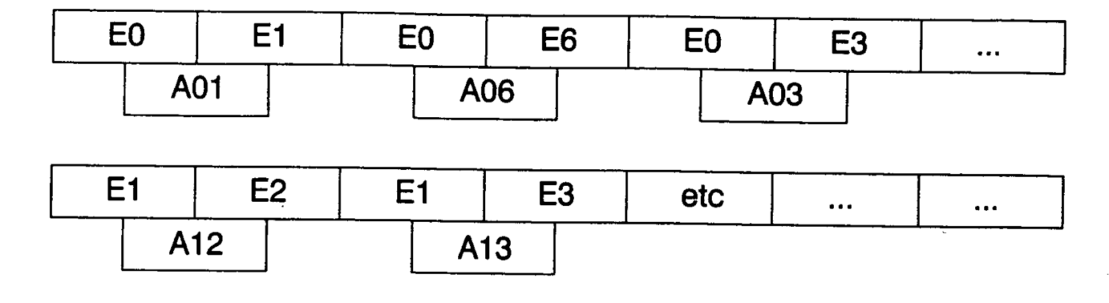
In the same way, Figure 3 shows a codification of graph, which has been codified by DNA, where represent vertex (in this case, cities) and represent edges (roads between cities). On the other hand, graph of Figure 1 would be called ‘G’ and its encoding could be seen in Figure 3, where A₀…A_n represents edges of graph and E₀….E_n represents cities or nodes of problem formulated.

Figure 3: Graph Codified by DNA.

Next step consists to arrange all the possible Hamiltonian paths inside of a seven vertices graph complete, by this reason, using cod-Inchrosil was created a set of 5040 DNA chains (factorial of seven), with strand length of 140 nucleotides (if problem has seven cities and each city has codification of 20 nucleotides, final strand length is 140 nucleotides). All this set of strand are organised by matrix form, because, it was more convenient to be able to approach a final three-dimensional chip, and in this way to emulate the nature, finally this matrix is called ‘CG’ in our experiment.

On the other hand, in set theory [26] is normally used to delimit the scope of a proposal, to compare if some object is part or not of one specific set, i.e. one set ‘S’ is defined as “YES”/ ”NO”, if and only if for some object α in included or not in ‘S’. In our case, we can compare each edge of ‘CG’ matrix with each specific edge in ‘G’ graph. All this operation can do in parallel way and the same time can obtain all edges are included in ‘G’ graph. Being each edge of ‘CG’ object need be compared with edge set proposal for programmer to determine which of these edges are included in ‘G’, remember, ‘CG’ is all possible solutions of the problem. As it is described in [24], Inchrosil is an electronic circuit allows storing all information of one pair of nucleotides by binary form, you can see Figure 4. This minimal unit allows create complex form or set of nucleotides (activating or not complementary chain), in our example all chains of ‘G’ graph and ‘CG’ matrix.

Figure 4: Inchrosil Unit

Above, we have described a parallel comparison between ‘CG’ matrix and ‘C’ graph to find all possible edges included in ‘C’. To be able to perform these comparisons in our experiment is necessary to use the philosophy of logical half-adders [27], carry-save adders (CSA) and Wallace trees. Highlight, for our experiment is removed carry option in massive comparison, doing direct additions of two inputs. On the other hand, following truth table of XOR gate, when two inputs are the same result, final result is 0, by this reason, in our experiment we have considered to invert all outputs, being 1 in all positive case and 0 in all negative case. Due to this approach, comparers were developed with XNOR gates to resolve the problem, by this reason; in our experiment, we have joined together 40 XNOR gates, where if each edge has 20 nucleotides, being 40 bits per edge and 80 bits of inputs, since it will be compared two by two. With this system, it is possible to create CSA without carry, where joining all XNOR gates would giving a unique result of 40 bits.

Finally, the system offered a 40 bits result, which was not optimum to specify one edge is the same or not, because final answer should be ‘yes’ or ‘no’ (i.e. 0 or 1). In this case, we needed a system to check all input and to generate only one output, by this reason, using only AND gates, we were able to create a system, which has 40 inputs and only one output, where system gives a ‘1’ as logical result, this result would mean that both edge are the same, on the other hand, if logical result is ‘0’, both edges are different. In case of positive result, edge is part of ‘G’ graph (which is a possible Hamiltonian path). 

This process could be parallel, by this reason, all comparer are distributed by one matrix form to compare by parallel way, all edge (two to two) in twice systems (‘G’ graph and ‘CG’ matrix). Highlight, with this system we can obtain if one edge is contained in ‘G’ graph solution, but with this sub-method do not indicate yet, if ‘G’ graph solution is a Hamiltonian Path, by this reason, in our experiment, we have used sub-method of Wallace trees methodology [28]. In general, they have same philosophy of Wallace Trees, but some specific customizations in their structure, i.e. we have created one for each sub-result of comparison (column of matrix). These systems are composed by OR gates, creating with this way, several levels as Wallace trees to find all possible coincidences between edges and chains.

The final objective is to find one chains where all edges have coincidences, in this case, we would have a Hamiltonian Path. That is possible because all outputs of OR gate system are connected with other system compose for AND gates and only one output, which indicates ‘YES’ or ‘NO’ the possible solution is Hamiltonian path. 

Finally, we can obtain a vector with n components (being n in our case, 5040 chains), where one element of vector has ‘1’ logical value, this element indicates is Hamiltonian path. In this case, we considered t_p as time to create all possible solutions, t_c as time to compare all edges of one component, t_f as time to compare all sub-results, t_a as additional time (delays in gates, communications, check final vector, etc.) and finally, n as number of components, we can formulated final time is T = t_p + n t_c + t_f + t_a, being this time close to polynomial order, because before times are considered in polynomial order. 

On the other hand, due modularity of the system, it is possible to create complex structures or system with huge number of nodes, because we can create circuit to solve partial solutions and later to join all solution to find final solution.

In Figure 5, we can see all circuit to calculate any Hamiltonian path of 7 cities, where the reference Figure 5-18 is ‘CG’ matrix with all possible Hamiltonian paths, the reference Figure 5-12 is the module, which compares edges between ‘CG’ and ‘C’, references Figure 5-15 and Figure 5-16 are logical gates to calculate similarity between DNA chains and finally, the reference Figure 5-20 is a vector with all comparison.

Figure 5: Hamiltonian Path Circuit

References

[1] Sanjeev Arora and Boaz Barak, Computational Complexity: A Modern Approach, Cambridge University Press, 2009.

[2] Hopcroft John E., Motwan Rajeev, Ullman Jeffrey D, Introduction to Automata Theory, Languages, and Computation, Prentice Hall, 2007.

[3] A. Gibbons, Algorithmic Graph Theory, Cambridge University Press, 1985.

[4] F. Harary, Graph Theory, Perseus Books, 1994.

[5] L. Euler, Solutio Problematis ad geometriam situs, 1736.

[6] E. W. Dijkstra, A note on two problems in connexion with graphs, Numerische Mathematik, p. 269–271, 1959.

[7] R. W. Floyd, Algorithm 97: Shortest Path, Communications of the ACM 5 (6), p. 345, 1962.

[8] S. Warshall, A theorem on Boolean matrices, Journal of the ACM, p. 11–12. 1962.

[9] John von Neumann, First Draft of a Report on the EDVAC, 1945.

[10] J. D. Markgraf, The Von Neumann bottleneck, 2007.

[11] Jordan Baumgardner, Karen Acker, Oyinade Adefuye and Samuel Thomas Crowley, Solving a Hamiltonian Path Problem with a bacterial computer, Journal of Biological Engineering, 2009.

[12] Leonard Max Adleman, Molecular computation of solutions to combinatorial problems, Science, p. 1021–1024, 1994.

[13] Liu W, Gao L, Liu X, Wang S and Xu J, Solving the 3-SAT problem based on DNA computing, 2003.

[14] Gheorghe P˘aun, Introduction to Membrane Computing, 2009

[15] Mihai Oltean, Solving the Hamiltonian path problem with a light-based computer, Natural Computing, 2008

[16] Gerald L. Thompson and Shared Singhal, A probabilistic polynomial Algorithm for solving a directed Hamiltonian path problem, 1983

[17] Omar M. Sallabi and Younis El-Haddad, An Improved Genetic Algorithm to Solve the Traveling Salesman Problem, World Academy of Science, Engineering and Technology, pp. 403-406, 2009

[18] Frank Rubin, a Search Procedure for Hamilton Paths and Circuits, Journal of the ACM, p. 576–80, 1974

[19] Richard Bellman, on a routing problem, Quarterly of Applied Mathematics, p. 87–90, 1958

[20] L. R. Ford Jr., Network Flow Theory, 1956

[21] E. F. Moore, The shortest path through a maze, Proc. Internat. Sympos. Switching Theory 1957, Part II. Cambridge, Mass.: Harvard Univ. Press, p. 285–292, 1959

[22] J. Y. Yen, An algorithm for finding shortest routes from all source nodes to a given destination in general networks, Quarterly of Applied Mathematics, p. 526–530, 1970

[23] Silvia, Jose Daniel and Carlos Llopis, DNA based in silicon (Inchrosil), International Journal of Scientific & Engineering Research, pp. 728-732, 2014.

[24] Silvia, Jose Daniel and Carlos Llopis, Electronic System for emulating the chain of the DNA structure of a chromosome. Spain Patent WO 2009/022024 A1, 19 Febrary 2009.

[25] Foreman, Matthew and Akihiro Kanamori, Handbook of Set Theory, 2010.

[26] M. Morris Mano, Digital Logic and Computer Design, Prentice-Hall, 1979

[27] C. S. Wallace, A suggestion for a fast multiplier, IEEE Trans. on Electronic Comp, 1964.

Computational Problems and its complexity

Any mathematical and computer problem could be classified according their inherent difficulty and its time necessary to solve the entire problem (Computational Time), this science area is called Computational Complexity Theory [1]. One computational problem could be viewed as a collection of instructions or equation, which is solved individually to find the entire solution of the problem; other people define one computational problem as some problem could be solved in a computer, both definitions are complementary to define a computational problem [2].

Computational and mathematical problem can divide in next groups:

• P Complexity: This group contains all problems can be solved in a deterministic machine and one polynomial time.
• NP Complexity: This group contains all problems can be solved in a non-deterministic machine and one polynomial time.
• NP Complete Complexity: This group contains all problems can be solved in a non-deterministic machine and not polynomial time.

On the other hand, there is other science area focused in resolving combinatorial problem by means of graph theory [3] [4], because any combinatorial problem could be converted to graph. In general, one graph can be defined as set of objects, where each object is connected with another object by links. Those connections are called edges and they can have direction or not inside of the path, making up directed or undirected graphs. On the other hand, each object is called vertex, as we said before, each vertex can join with other vertex by one or several edges with different vertex, inclusive itself. The graphs can have several classifications depending of different characteristics (weight edges, number of connections, direction, etc).

One pioneer inside of graph theory and topology was Leonard Euler, who in 1736 shows “the Seven Bridges of Königsberg problem” [5], highlight, in that period, Königsberg was Prussian city (now Kaliningrad, Russia) with seven bridges, over the Pregel River. The Euler’s problem formulates as one pedestrian is possible to walk through the city that would cross each bridge once and only once. This problem is an excellent combinatorial problem to convert in a graph form, because each part of the city is possible to represent as element of graph. Later, the Irish mathematician, William Rowan Hamilton and the British mathematician, Thomas Kirkman [6] formulated mathematically in 1800’s the Travelling Salesman Problem (next lines, we can called as TSP), in same time, it was formulated Hamiltonian Path Problem (following HPP), one of the most mathematical complex problems in graph theory, impossible to do in deterministic algorithm with huge number of elements.

In XX century, Edsger Wybe Dijkstra published one algorithm [7], which is a graph search algorithm that solves the single-source shortest path problem for a graph with non-negative edge path costs, making a shortest path tree, mainly this algorithm is often used in routing task or part of other graph algorithms. Later, Robert W. Floyd and Wharshall [8] [9] modified Dijkstra’s algorithm, which compares all possible paths through the graph between each pair of vertices to find shortest paths in weighted graph with positive or negative edge weights. Finally, From Dijkstra to now, there are lot algorithms or modifications of these algorithms to calculate shortest path or any route.

On the other hand, today the current computing systems are based on a sequential technology established by John Von Neumann [10] [11] in the middle of the last century. These sequential computers are good at resolving mathematical problems, because they have a powerful arithmetic unit inside, which can do complex operations with binary arithmetic. Also, these computers have difficulties with so-called turnkey problems, where all possible solutions should check to find a final solution, by this reason; these systems lost a huge time in the preparation all possible solution and later check one per one, being their computational time close to exponential or logarithmic order. One perfect example is HPP, which with a few nodes or cities, any system can solve it, but when the number or cities or nodes is huge, this problem cannot solve in polynomial time or similar, by this reason, there is not deterministic algorithm to solve the problem.

At the moment, scientific community can solve these problems with the construction of parallel computers or supercomputers, which divide and share each part of the problem between all different nodes of the system. This methodology can reduce the computing time close to polynomial, but finally, these solutions consume many resources in communications between a lot interconnected nodes, which are normally sequential computers. There are other initiatives to solve combinatorial problems, for example, using organic materials, we can find bacterial computer to solve HPP [12], on the other hand, using DNA to resolve HPP by Prof. Adleman [13], the 3-SAT problem using DNA [14], implementations in membrane computing [15] and others organic solutions.

In this way, using organic materials (in particular DNA), in 1994, Professor Adleman formulated a new alternative for programming with organic DNA, using huge mathematical knowledge about computation with DNA and last advances in DNA. He created a DNA computer to solve HPP with seven nodes, using organic material. Which this experiment, he demonstrated that NP-Complete problems could be resolved in a computational time very close to the polynomial, being very close to find one solution of universal problem of PNP.

With this experiment, Prof Adleman shows the huge potential of DNA computing, breaking walls using organic material in computer science. Also, DNA Computing has huge potential to solve complex problems, but this methodology of computing contains certain barriers. For one side, implicit characteristics of material used (organic DNA), because is mainly perishable and long of time it dies. Other side, DNA machines are difficult to integrate in other environments as organics or silicon system, mainly in communication between them, by this reason, these systems are limited only for scientific environments and theoretical formulations.

Finally, in other field as optical, we can find works as solving HPP with light-based computer [16], on the other hand, using mathematical-theoretical equation for solving HPP [17], also with genetic algorithms to solve TSP [18] or by other systems or methodologies in different science areas.


References

[1] Sanjeev Arora and Boaz Barak, Computational Complexity: A Modern Approach, Cambridge University Press, 2009.

[2] Hopcroft John E., Motwan Rajeev, Ullman Jeffrey D, Introduction to Automata Theory, Languages, and Computation, Prentice Hall, 2007.

[3] A. Gibbons, Algorithmic Graph Theory, Cambridge University Press, 1985.

[4] F. Harary, Graph Theory, Perseus Books, 1994.

[5] L. Euler, Solutio Problematis ad geometriam situs, 1736.

[6] E. W. Dijkstra, A note on two problems in connexion with graphs, Numerische Mathematik, p. 269–271, 1959.

[7] R. W. Floyd, Algorithm 97: Shortest Path, Communications of the ACM 5 (6), p. 345, 1962.

[8] S. Warshall, A theorem on Boolean matrices, Journal of the ACM, p. 11–12. 1962.

[9] John von Neumann, First Draft of a Report on the EDVAC, 1945.

[10] J. D. Markgraf, The Von Neumann bottleneck, 2007.

[11] Jordan Baumgardner, Karen Acker, Oyinade Adefuye and Samuel Thomas Crowley, Solving a Hamiltonian Path Problem with a bacterial computer, Journal of Biological Engineering, 2009.

[12] Leonard Max Adleman, Molecular computation of solutions to combinatorial problems, Science, p. 1021–1024, 1994.

[13] Liu W, Gao L, Liu X, Wang S and Xu J, Solving the 3-SAT problem based on DNA computing, 2003.

[14] Gheorghe P˘aun, Introduction to Membrane Computing, 2009

[15] Mihai Oltean, Solving the Hamiltonian path problem with a light-based computer, Natural Computing, 2008

[16] Gerald L. Thompson and Shared Singhal, A probabilistic polynomial Algorithm for solving a directed Hamiltonian path problem, 1983

[17] Omar M. Sallabi and Younis El-Haddad, An Improved Genetic Algorithm to Solve the Traveling Salesman Problem, World Academy of Science, Engineering and Technology, pp. 403-406, 2009

[18] Frank Rubin, a Search Procedure for Hamilton Paths and Circuits, Journal of the ACM, p. 576–80, 1974

[19] Richard Bellman, on a routing problem, Quarterly of Applied Mathematics, p. 87–90, 1958

[20] L. R. Ford Jr., Network Flow Theory, 1956

[21] E. F. Moore, The shortest path through a maze, Proc. Internat. Sympos. Switching Theory 1957, Part II. Cambridge, Mass.: Harvard Univ. Press, p. 285–292, 1959

[22] J. Y. Yen, An algorithm for finding shortest routes from all source nodes to a given destination in general networks, Quarterly of Applied Mathematics, p. 526–530, 1970

[23] Silvia, Jose Daniel and Carlos Llopis, DNA based in silicon (Inchrosil), International Journal of Scientific & Engineering Research, pp. 728-732, 2014.

[24] Silvia, Jose Daniel and Carlos Llopis, Electronic System for emulating the chain of the DNA structure of a chromosome. Spain Patent WO 2009/022024 A1, 19 Febrary 2009.

[25] Foreman, Matthew and Akihiro Kanamori, Handbook of Set Theory, 2010.

[26] M. Morris Mano, Digital Logic and Computer Design, Prentice-Hall, 1979

[27] C. S. Wallace, A suggestion for a fast multiplier, IEEE Trans. on Electronic Comp, 1964.

 

First video of Threellop Nanotechnology

Threellop in CLARCIEV 2009 (Colombia)

Home Page